Hi there! This and the next blog post aim at intuitively explaining CMA-MEGA and some of its variants. “CMA” stands for CMA-ES, and “MEGA” stands for MAP-Elites via a Gradient Arborescence, so the name gives away two constituent parts of the algorithm. If you are unfamiliar with CMA-ES, you can check out my 3-part series (part 1, part 2, part 3), but no need to worry too much about it, because CMA-ES is optional and can be substituted with any random sampling. The central piece here is actually MAP-Elites via a Gradient Arborescence (MEGA), which presents a new way to use gradient search on quality and diversity simultaneously. The idea was proposed in Fontaine, Matthew, and Stefanos Nikolaidis (2021) and further developed in Tjanaka, Bryon, et al. (2022).
If you are like me, you are probably confused by the keyword gradient. Isn’t being black-box one of the key characters of evolution strategies, and arguably the Quality-Diversity family in general? Normally we just send a genome into evaluation and get back its fitness (and behavior descriptor) without knowing the evaluation process. If we don’t know a function how can we calculate a gradient? But even before this, there’s another major question to be answered:
What does gradient even mean in the context of MAP-Elites?
Remember that in MAP-Elites (Mouret, J. B., & Clune, J. (2015)), we try to get an archive of diverse solutions(parameterized by genome) each accomplishes the objective well, but also does it in a different way. We measure how well the objective is accomplished with fitness, and we indirectly measure the difference among solutions with behavior descriptors(BD), where both measures are defined according to how we want our solutions to behave. So summing up:
- We want our genomes to discover as many BDs as possible
- We want the genome in each BD to have as high a fitness as possible
It makes sense to use gradient (assuming we know the gradient) on the second objective (fitness), since we are familiar with using gradient in the context of optimization. For example, assuming we know a function $y = f(x_1, x_2)$ that maps from the genome $[x_1, x_2]$ to fitness $y$, then the gradient of $y$ w.r.t. $x_1$ and $x_2$, indicates, at a certain value of $x_1$ and $x_2$, which direction we should travel on the $x_1$-$x_2$ plane in order to get the largest increase in fitness.
However, it’s not obvious how we can use gradient to encourage our genomes to discover more BDs – what are we trying to maximize here? For a start, it doesn’t make sense to simply calculate the gradient of each BD measure w.r.t. genome, since that would only encourage solutions to have high values within each BD measure, which actually makes the solutions more alike! For example, in the problem of quadruped locomotion where there are 4 BDs recording the proportions of time $[0, 1]$ each leg touches the ground, using the aforementioned approach will likely result in most solutions having around $0.9$ or $1$ BD values for all 4 legs, whereas what we really want are diverse solutions spanning the entire BD range.
So what are the alternatives? One option is to define an explicit novelty measure, such that we can compute the gradient of novelty w.r.t. genome and maximize novelty. For example, ME-ES defines novelty as the Euclidean distance between a genome’s BD and its nearest neighbors (kinda similar to NSLC). For another (more complex) example, QD-PG breaks down a genome’s evaluation into state-action pairs, and defines novelty as the sum of differences between this genome’s visited states and the most similar states visited by other genomes.
But in this blog, I wish to focus on another approach to use gradient on diversifying BDs. What if we calculate a weighted sum of BDs like this: $\Sigma_{j}^k c_j BD_j = c_0 BD_0 + c_1 BD_1 \ldots + c_k BD_k$, and maximize this sum by calculating its gradient w.r.t. the genome? The trick here is that we can define how much we want to maximize/minimize each BD measure by defining its coefficient. For example, we can encourage the genome to achieve a small $BD_0$ by setting $c_0$ negative. Generally speaking, BD measures paired with large coefficients will be more strongly encouraged to be large and vice versa, so by defining a list of coefficients $c_0 \ldots c_k$, we define a direction we want to explore in BD space!
 We can change the gradient’s direction by changing coefficients to each term in a function; run
 coeffs_demo.py to play around!
Having just one direction to explore doesn’t result in diverse solutions by itself, since we’ll just end up with a variant of the all-high-BDs case. So here comes the second trick: What if we generate a new random set of $c_0 \ldots c_k$ (i.e. a new exploration direction) every few iterations? By doing this, we accomplish a similar effect as the random direction emitter in CMA-ME (Fontaine et al. (2020)). The direction (i.e. coefficients) can of course be simply random, but there are scenarios where some directions should be favored over others. For example, if the BD cells along direction $A$ have already been well-explored, whereas those along direction $B$ are empty, then intuitively direction $B$ should be favored over $A$. To allow the algorithm to learn this information, we can use CMA-ES to evolve the coefficients $c_0 \ldots c_k$, and use the improvement score ranking rule during its update (similar to CMA-ME).
But why stop here? If we are trying to maximize the fitness, and we are also trying to maximize the weighted sum of BDs, then why not maximize them together by introducing another coefficient to fitness and adding it into the weighted sum like this:
$ |c_0|Fitness + \Sigma_{j=1}^{k+1} c_j BD_{j-1} = |c_0|Fitness + c_1BD_0 + c_2BD_1 \ldots + c_{k+1}BD_k $
$c_0$ is introduced to allow the gradient search to choose how much it cares about fitness relative to BD exploration. But since we never want to search for low fitness, $|c_0|$ is kept positive. (Edit: I later learned this was actually false, because in the paper c0 was indeed NOT kept positive with absolute value. I think this was because the optimizing pressure on fitness was already being applied through the cell replacement procedure in MAP-Elites, so adding extra pressure through forcing c0 to be positive would have been redundant. Additionally, since absolute value would essentially reverse the sign, it would also break the continuity in QD space.) Taking the gradient of this weighted sum w.r.t. genome gives us:
$ |c_0|\nabla_{\theta}Fitness + \Sigma_{j=1}^{k+1} c_j \nabla_{\theta}BD_{j-1} $
where $\nabla_{\theta}Fitness$ represents the gradient of fitness w.r.t. genome, and $\nabla_{\theta}BD_{k}$ represents the gradient of k-th BD measure w.r.t. genome. Assuming we have these gradients, which we will come to in a minute, we can update the genome with:
$ \theta’ = \theta + |c_0|\nabla_{\theta}Fitness + \Sigma_{j=1}^{k+1} c_j \nabla_{\theta}BD_{j-1} $
So the workflow goes like this:
- Randomly select a $\theta$ from the MAP-Elites archive
- Select $c_0 \ldots c_k$ (optionally with CMA-ES)
- Evaluate genome $\theta$ (if using CMA-ES, need to evaluate multiple $\theta$ each corresponding to a coefficient set generated by CMA-ES)
- Update MAP-Elites archive (if using CMA-ES, need to update CMA-ES as well)
- Given $\nabla_{\theta}Fitness$ and each $\nabla_{\theta}BD_{k}$, as well as the coefficients, calculate the overall gradient
- Update $\theta$ with the calculated gradient
- Return to step 2 if need to explore a new direction, otherwise return to step 3
The idea of calculating the gradient for, and hence maximizing, the weighted sum of fitness and BDs, in order to simultaneously maximize fitness and explore a selected direction in BD space, is referred to as MAP-Elites via a Gradient Arborescence (MEGA). However, what we just described is only half the story. Now that we know how to use gradient and what to maximize in MEGA, we need to return to a question we raised at the beginning:
But how to get gradients?
In the workflow above we assumed we knew $\nabla_{\theta}Fitness$ and and each $\nabla_{\theta}BD_{k}$, but how do we get them exactly? If we know a well-defined function that maps from the genome to fitness and each BD measure, then obviously we can just calculate the gradients with good’ol maths. This might be the case for some special problems. For example, in Fontaine, Matthew, and Stefanos Nikolaidis (2021), one of the experiments they considered was learning the inverse kinematics of a robotic arm, where genome was the set of joint positions, fitness was based on how much joint angles vary, and the 2 BDs were x and y coordinates of the arm’s hand. In this case, we have the well-defined function since we know forward kinematics, so the gradients was just the jacobian.
However, more often than not, we do not have access to such functions (or why else would we “evaluate” a genome?). In this case all we have is a black-box procedure we know nothing about, except it returns us with fitness and BDs after being fed a genome. Here we cannot calculate the gradients, but we can actually estimate them.
The intuition is simple. Gradient is about indicating the parametrical direction of the locally steepest increase, e.g. how to change the genome to get the locally largest increase in fitness. If we have an unknown function $y = f(x_1, x_2)$, and we want to know how to change $x_1$ and $x_2$ to best increase $y$ at the current location $x_1=x_1’, x_2=x_2’$, why not take some samples around $x_1’, x_2’$, and see how their evaluations $y_{noise} = f(x_1’+noise_1, x_2’+noise_2)$ compare to the current evaluation $y’ = f(x_1’, x_2’)$? Some $y_{noise}$ may have higher evaluations, so we know their corresponding noises represent a good direction to change $x_1’$ and $x_2’$ if we want to increase $y$, and vice versa. If you know CMA-ES, this intuition might sound familiar, but although CMA-ES also relies on probing around the centroid to get a good feeling on update direction, it doesn’t explicitly give a gradient estimate. To estimate a gradient, we need to borrow from NES the formula:
$ \nabla_{\theta} E_{\epsilon \sim N(0, I)} F(\theta + \sigma \epsilon) = \frac{1}{\sigma} E_{\epsilon \sim N(0, I)} \{ F(\theta + \sigma \epsilon)\epsilon \} \approx \frac{1}{n\sigma} \Sigma_{i=1}^n F_i \epsilon_i $
According to this formula, we sample $i$ times from a standard normal distribution, and use the samples as noises to add to our current genome $\theta$, which gives us $i$ perturbed genomes, and after evaluated, $i$ fitnesses. Then to get the gradient, we just scale each noise $\epsilon_i$ with its corresponding fitness $F_i$, average all scaled noises. $\sigma$ is a hyperparameter determining how large do we scale the noises. For very rugged fitness landscapes, we may want to tune $\sigma$ down. $n$ is another hyperparameter deciding how many perturbed genomes we sample to estimate the gradient; more samples usually means better estimate, but at the cost of more genomes to evaluate. NES defined this gradient estimate for fitness, but the procedure is the same for BDs. With this we can estimate the gradients of fitness and each BD w.t.r. genome. After adding gradient estimate, the workflow looks like this:
- Randomly select a $\theta$ from the MAP-Elites archive
- Select $c_0 \ldots c_k$ (optionally with CMA-ES)
- Evaluate genome $\theta$ (if using CMA-ES, need to evaluate multiple $\theta$ each corresponding to a coefficient set generated by CMA-ES)
- Update MAP-Elites archive (if using CMA-ES, need to update CMA-ES as well)
- Generate perturbed genomes, evaluate, and estimate $\nabla_{\theta}Fitness$ and each $\nabla_{\theta}BD_{k}$
- Given $\nabla_{\theta}Fitness$ and each $\nabla_{\theta}BD_{k}$, as well as the coefficients, calculate the overall gradient
- Update $\theta$ with the calculated gradient
- Return to step 2 if need to explore a new direction, otherwise return to step 3
That pretty much sums it up! Just a few minor details to help with the convergence:
- As a standard practice, gradients need to be normalized, i.e. divide by L2-norm.
- Rank normalization may be applied on sample fitnesses during gradient estimate. Rank normalization simply means sorting all fitnesses, and using the sorting indices in place of raw fitnesses. This prevents an outlier fitness from having too much effect on the gradient estimate.
- Also during gradient estimate, mirror sampling may be used to reduce sampling variance. This is a bit harder to explain so I recommend checking out Tjanaka, Bryon, et al. (2022) Appendix Algorithm 4.
Implementation
Codes available here! Go to the bottom of agent.py and comment/uncomment according to instruction to either train an agent or display the current one. Below shows the result after 6000 generations. I’ve found that CMA-MEGA(ES) is more economic with the number of generations than CMA-ME, but each generation takes longer because of the additional evaluations required by the gradient estimate.
 QDAnt best gait after 6000 generates of CMA-MEGA(ES)
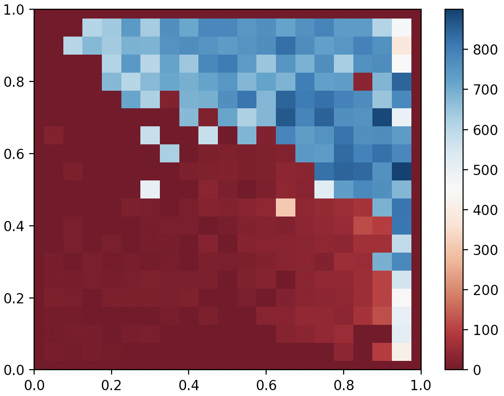 QDAnt partial archive after 6000 generates of CMA-MEGA(ES)
On this specific problem, CMA-MEGA(ES) seems to have comparable performance with CMA-ME. But I think CMA-MEGA has superior scalability to CMA-ME, because regardless of how many parameters the genome has, CMA-MEGA only explores on the Fitness-BD space, which is often of much lower dimensionality than genome. Here our genome only consists of 24 parameters, but I believe CMA-MEGA will shine when we start training neural networks parameterized by much higher dimensionality genomes. I’ll try that in the next blog, stay tuned!