Hi there! This blog post aims to be a gentle introduction to MAP-Elites algorithm. We’ll look at how MAP-Elites works, what motivated its development, why it might be a promising direction of research, and we’ll end with a demo where we implement a simple MAP-Elites and apply it on the QDgym Ant environment.

This blog post assumes some degree of familiarity with evolutionary algorithms, so I recommend checking out my blog post on simple ES. You don’t need to go over the entire blog; just make sure you understand the following:

Fundamentally, ES works by generating individuals and updating the generator in a way that relies more on high-fitness individuals, such that the generator is more likely to produce higher-fitness individuals next time.
One way to generate individuals is through sampling from a multivariate normal distribution.
If we use a multivariate normal distribution as the generator, we can update its mean to improve the generator.
We can update the mean by resetting it to the mean of a subset of high-fitness individuals (also known as elites).
For simplicity we may neglect updating the covariance matrix in this blog post; simply use $diag(\sigma)$ throughout evolution where $\sigma$ is defined by user as a hyperparameter.

All in all, a simple evolution can be defined in the following pseudocode:

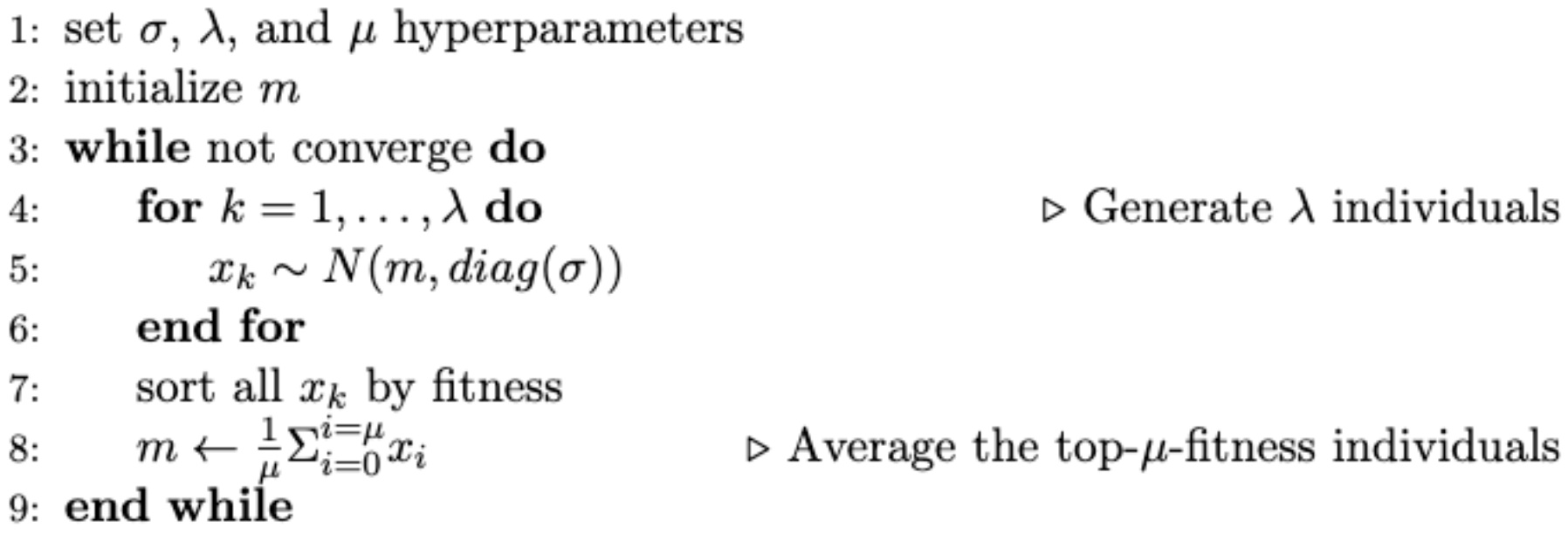simple-ES pseudocode

Problem: Local Optima

You likely have heard of the term “local optima” if you’ve worked with anything related to optimization and machine learning. Local optima are points in the parameter space that have higher fitness than their immediate surroundings, but are not the best over the entire space (hence “local”, as opposed to “global”, optima). A greedy optimizer that over-exploits local improments is likely to find local optima instead of the global optimum, and therefore gradient-based methods are famously vulnerable to local optima. The simple-ES that we just proposed also falls victim to this problem.

Simple-ES finds high-fitness neighborhood to the top, even though global optimum is to the buttom

In the demonstration above, there’s a path of steadily-increasing fitness that leads to the local optimum to the top. By comparison, the global optimum to the bottom is harder to reach because there’s a valley between our starting point and the optimum where fitness temporarily drops. Our simple-ES got discouraged by the low-fitness valley, and thus failed at finding the global optimum.

One Solution: Niching

In the simple-ES above, each individual competes against every other individual, regardless of how far said individual is from it in the parameter space. Since all individuals compete against all other individuals globally, we call this approach global competition. This seems intuitive enough, until we remember this is not how evolution works in nature, where competition is often confined within local neighborhoods. For example, cheetahs in Africa don’t compete against penguins in Antarctica. Even when inhabiting the same environment, genetically different species tend not to directly compete against each other (excluding prey-preditor relationship). Local competition allows each species to explore the means of survival in its own way. This enabled great diversity among creatures inhabiting the world today. More crucially, maintaining multiple exploration directions allows evolution to have “backups”, such that if one species gets stuck with a local optimum, evolution can continue exploring with other more successful species.

Taking inspiration from nature, we can modify our simple-ES such that any individual only competes against others that are similar to it. The idea is known as niching, as shown below:

Niching creates local pockets of competition, and therefore maintains multiple exploration directions

How to measure similarity between individuals?

Ok, so we’ve decided to only allow competition among similar individuals, but how do we calculate the similarity between two individuals? An obvious method could be to calculate the Euclidean distance in parameter space between two individuals. Unfortunately, this method is insufficient for more complex evolution problems, such as when evolving a neural network. This is demonstrated in the competing convention problem:

Competing Convention Problem; image from Stanley, K. O., & Miikkulainen, R. (2002)

In the illustration above, both networks have learned sub-functions $A$, $B$, and $C$, but since there’s no convention specifying which part of neural network should learn which sub-function, the two networks become permutations of one another. From the perspective of Euclidean distance between network weights, the two networks would have appeared to be different, even though they learn the same sub-functions and therefore are practically the same. Generally speaking, competing convention problem describes the observation that the parameter/function maps are usually non-injective because identical function can be encoded in many different ways, so it’s difficult to compare individuals by their parameters. Another issue with comparing parameters is computational complexity. Taking neural networks for example, the number of parameters(weights) for one individual grows exponentially with network size, so computing distances between every pair of individuals every generation can be forbiddingly slow.

The aforementioned reasons against comparing individuals by their parameters introduce us to one of the core concepts in MAP-Elites: instead of comparing parameters, why not simply compare the end results, i.e, behaviors? To quote the well-known duck test:

If it swims like a duck, and quacks like a duck, then it probably is a duck. (The subtext being that we usually don’t need DNA test to know a duck is a duck)

I think that sums up the idea pretty well. We decide on a few behavioral descriptors we care about, and compare individuals according to how much their bahavioral descriptors differ. For example, if we are evolving neural networks to move around in the mujoco Ant environment, then we can compare the individual networks by the xyz displacements of their ants, in which case the xyz displacements would be our behavioral descriptors. Note that comparing behavioral descriptors does not require parameter/function mapping and therefore circumvents the competing convention problem. Moreover, xyz displacements are just 3 numbers to compare – much easier than comparing thousands of neural network weights!

How to implement local competition?

So far we have seen how local competition (i.e. allowing only similar individuals to compete against each other) helps ES maintain multiple exploration directions and hence overcome local optima, and why comparing behaviors is preferred over comparing parameters when determining individuals’ similarity. Now let’s discuss about the implementation of local competition.

There are two general lines of thought. The first is known as fitness sharing. The name is self-explanatary: each individual has its raw fitness discounted according how many other individuals lie within a certain distance from it, such that each individual is encouraged to distance itself from the others and find its own niche. I won’t go into too much detail because MAP-Elites go by the other approach.

The other approach is known as crowding. It’s simpler than fitness sharing and probably similar to your first idea on how to implement local competition – individuals within a certain distance (and only within a certain distance) to one another compete such that only one winner is left in that neighborhood. This first idea requires computing distance between every pair of individuals, which is costly. MAP-Elites simplifies the calculation by discretizing the behavioral descriptor space into grids. Individuals that fall into the same grid are considered similar and compete with each other leaving one winnder in that grid, as shown below:

Image from Notebook for the MAP-Elites tutorial

This is also where the nomenclature of MAP-Elites comes in – because at the end of evolution we’ll have an archive of high-fitness individuals each accomplishing the target task through behavior decribed by its behavior descriptor niche (a “map” of “elites”, you might say).

Summary

This concludes our discussion on the concepts behind MAP-Elites. In the end, MAP-Elites is actually a relatively simple algorithm:

Image from Mouret, J. B., & Clune, J. (2015)

Just keep the following in mind when implementing MAP-Elites:

Initialize a table whose indexing dimensions are the behavior descriptors you’ve selected.
For each individual generated, check which archive grid the individual falls into; if the grid is non-empty, replace the previous occupant only if the new individual has higher fitness; if the grid is empty then simply put the individual in.
There’s no strict restriction on how to generate individuals. You may crossover or mutate individuals from the archive (for which you’ll need a partially filled archive – so you’ll probably need to implement a warmup phase), or you may generate individuals through some external mechanism and use the archive only for storing elites.
Keep evolving and filling/updating the archive until you have a good enough individual in any of the grids.

Application

MAP-Elites can been seen as part of the recent trend (…ok, maybe not that recent) in evolution algorithm community to favor exploration, i.e. focus on generating novel individuals even if they may not have the highest fitness. Lehman, J., & Stanley, K. O. (2008) famously demonstrated that in certain tasks with deceptive/delayed/sparse reward (maze navigation in this case), optimizing for novelty alone while neglecting performance can actually be a valid approach! It was also argued in Lehman, J., & Stanley, K. O. (2011) and Salimans, T., et al. (2017) that the density of high-performing solutions is often high enough and the reward structure deceptive to merit exploration over exploitation. The importance of exploration justifies the emergence a family of evolution algorithms called Quality-Diversity(QD) algorithms, which search for a set of high-performing and distinct solutions rather than just one best solution. MAP-Elites belongs to this family, and aside from MAP-Elites which explores the search space indirectly, another major sub-family of QD algorithm is represented by Novelty Search with Local Competition(NSLC), which actively optimizes for novelty along with fitness using multi-objective optimizer algorithms such as NSGA-II.

MAP-Elites can also be applied for purposes other than optimization. The elite solutions stored in its archive can be used as backups in case of damage recovery or reality gap (Cully, A., et al. (2015), Tarapore, D., et al. (2016)). Another clever use of the elite solutions is to define behavior descriptors in a way that allows them to be combined to accomplish arbitrary behavior; in this case the archive serves as an approximate inverse dynamics model (Chatzilygeroudis, K., et al. (2016), Duarte, M., et al. (2017)).

Evolving a controller for Ant robot

Conveniently, QDgym already defines a gym environment that’s similar to mujoco Ant and returns behavior descriptor needed for MAP-Elites, so we’ll use that for the demo. Just like the mujoco Ant, QDgym Ant is a spider-like robot that has 4 legs each driven by 2 positional joints, making 8 inputs each in range [-1,1]. Input 1 bends the joint towards its maximum angle (I’m not entirely sure but I think it’s PID-controlled). Reward (fitness) is given according to how far the robot has travelled along the x-axis, as well as a range of minor factors such as joint swing, remaining upright etc.. The behavior decriptor used in QDgym is a 4-vector specifying proportions of time each leg touches the ground (you may try to define your own behavior descriptor if you are familiar enough with the PyBullet simulator).

The codes can be found here. Install QDgym and run agent.py to evolve a controller for QDgym Ant. I plan to go over the codes later in a video.

On my 2017 Macbook Pro with no GPU acceleration, running 10000 generations took about 20 minutes, and below I show the highest fitness “gait” as well as a partial archive visualizing only the first two dimensions (behavior descriptor is 4D in this case). Ok…not exactly convincing performance, but I’ve made modifications since then, and the result with CMA-ME looks much better!

QDAnt best gait after 10000 generates of MAP-Elites

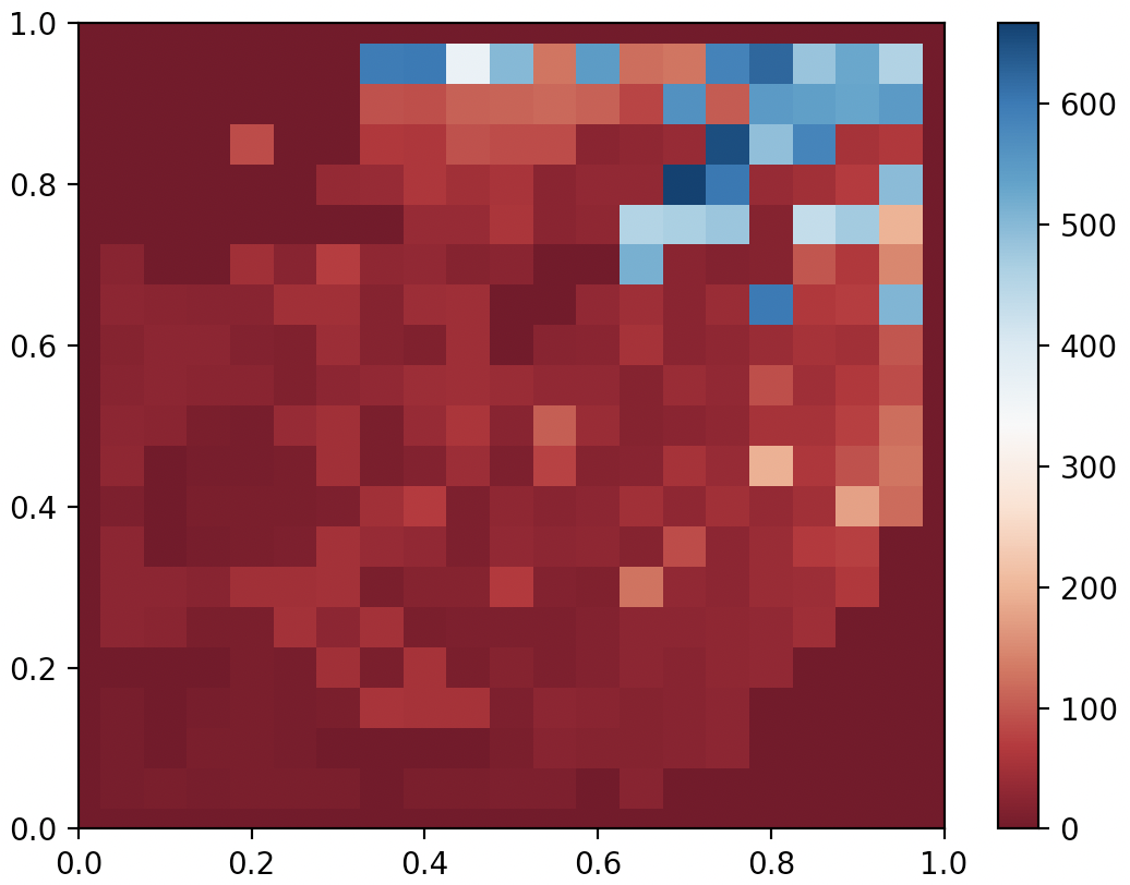QDAnt partial archive after 10000 generates of MAP-Elites