Welcome back! Previously in part 2 we looked at why and how CMA-ES de-coupled step size $\sigma$ and direction $C$. Here in part 3 we will discuss the mechanisms by which each is adapted independently.

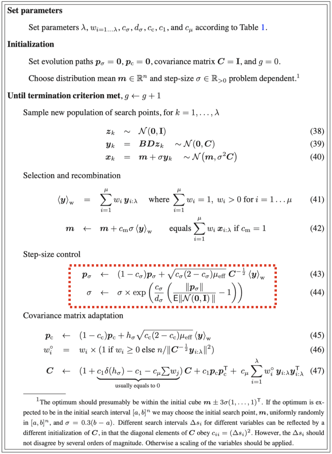pseudocode from The CMA Evolution Strategy: A Tutorial

Adapting step size $\sigma$

What can we learn from evolution path $p_{\sigma}$?

We saw in part 2 how the mean $m$ of the distribution was iteratively updated according to the weighted average of individuals, which were in turn sampled from a distribution centered around the previous mean. Let’s consider an evolution path consisted of all means seen so far, $m_0, m_1, \ldots, m_g$, and the overall update $m_0 \to m_g$, and let’s think about what the length of the overall update, $\lVert m_0 \to m_g \rVert$, tells us about the step size we’ve been using. Below shows 3 scenarios:

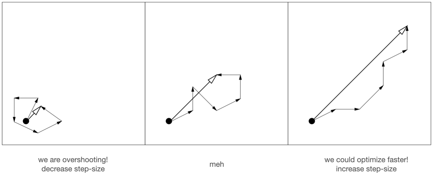How $m$ has been updating: 3 scenarios

As shown on the left, if $\lVert m_0 \to m_g \rVert$ is small, it’s probably indication that the directions of past updates $m_0 \to m_1, m_1 \to m_2, \ldots$ don’t align, and we’ve just been jumping back and forth around the optimum. This is the scenario where we’d want to decrease step size and let the algorithm converge. On the contrary, if $\lVert m_0 \to m_g \rVert$ is big as shown on the right, it’s probably indication that the past updates align in direction. In this case we’d want to increase step size because we know the direction is a good and larger updates give us faster optimization!

By this line of thinking, if we maintain a rolling sum of past mean update vectors, which, by the way, we get each generation as $y_w$ from the recombination step, we’d know to decrease step size if the length of the overall vector is small, and increase if large. But in order to decide whether the length is “large”, we need to reference it against something. In this case, CMA-ES uses the expected length of random sample $E \lVert N(0, I) \rVert$. Conveniently, this is a constant that depends on the dimensionality of sampling, i.e. number of parameters to be optimized, and thus can be computed at the start and reused each generation. With this reference, we have $exp(\frac{\text{length of overall update}}{E \lVert N(0, I) \rVert} - 1)$. Obviously, if the length of overall update is smaller than reference, then this scaling factor becomes smaller than 1 and the step size is downscaled.

How can we build up evolution path $p_{\sigma}$?

Let’s now talk about the update formula for the aforementioned “rolling sum”. You might be expecting something like this for the formula:

$ p_{\sigma} = (1 - c_{\sigma})p_{\sigma} + c_{\sigma}y_w $

where $p_{\sigma}$ is the accumulator, $y_w$ is the weighted average of $y_k \sim N(0, C)$, i.e. the update vector, and $c_{\sigma}$ controls the learning rate. But the actual update formula contains a few more things:

$ p_{\sigma} = (1 - c_{\sigma})p_{\sigma} + \sqrt{c_{\sigma}(2 - c_{\sigma})\mu_{eff}}C^{-\frac{1}{2}}y_w $

Firstly, $y_w$ is premultiplied with $C^{-\frac{1}{2}}$ because as the CMA-ES paper p21 puts it,

… $C^{(g)^{-\frac{1}{2}}}$ makes the expected length $p^{(g+1)}_{\sigma}$ independent of its direction

and we need $p_{\sigma}$ to be directionally independent because we will be comparing it against $E \lVert N(0, I) \rVert$, which is a directionally independent measure.

Secondly, $C^{-\frac{1}{2}}y_w$ is further scaled with $\sqrt{c_{\sigma}(2 - c_{\sigma})\mu_{eff}}$ because $y_w$ comes (albeit indirectly) from sampling, and thus the variance of $p_{\sigma}$ accumulates when we add the $C^{-\frac{1}{2}}y_w$ term every generation. The $\sqrt{c_{\sigma}(2 - c_{\sigma})\mu_{eff}}$ factor makes sure the variance of $p_{\sigma}$ stays the same.

$\mu_{eff}$ is defined as the ratio between the L1-norm squared and L2-norm of recombination weights, i.e. $\mu_{eff} = \frac{(\Sigma_{i=1}^{\mu}abs(w_i))^2}{\Sigma_{i=1}^{\mu}w_i^2} = \frac{1}{\Sigma_{i=1}^{\mu}w_i^2}$ (the weighst are normalized and $\Sigma_{i=1}^{\mu}abs(w_i) = 1$). With this knowledge, you can try to work out the maths of $\sqrt{c_{\sigma}(2 - c_{\sigma})\mu_{eff}}$ yourself! (Hint: $Var(aX + bY) = a^2Var(X) + b^2Var(Y)$ more hints on the CMA-ES paper p17)

Adapting direction $C$

That leaves us with just one more section to explain! In part 2 I mentioned that update step size $\sigma$ and direction $C$ would be updated differently. We just saw how to update $\sigma$; now let’s look at how $C$ updates and how is the mechanism different.

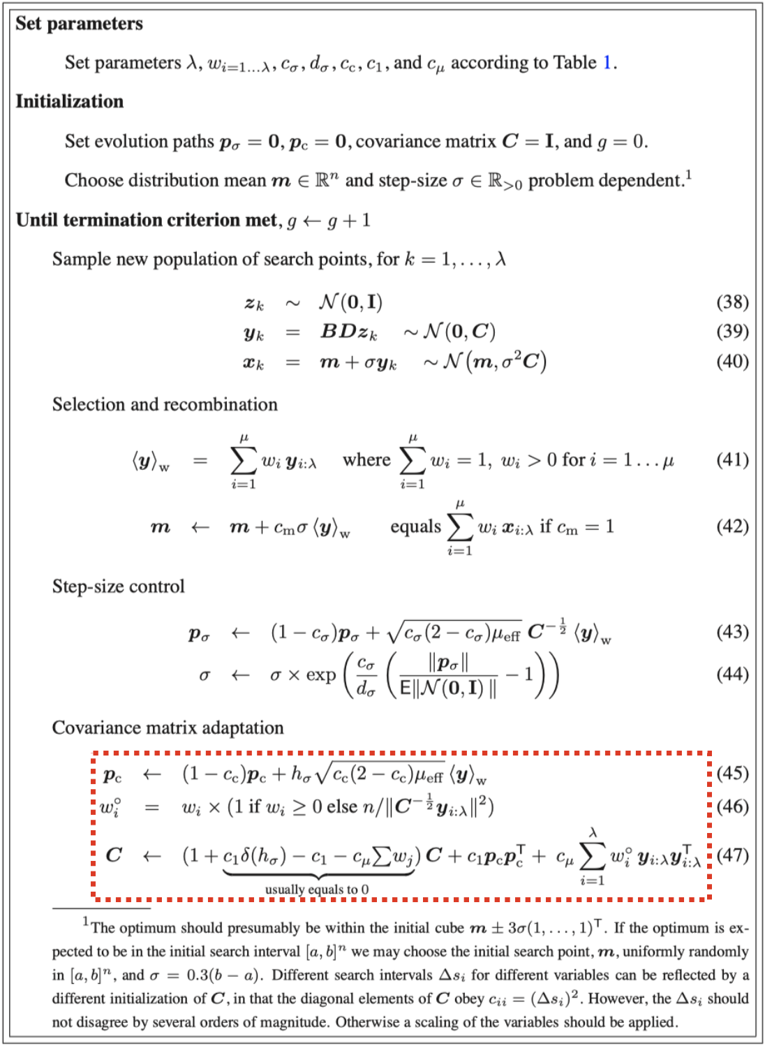pseudocode from The CMA Evolution Strategy: A Tutorial

If we look at the overall update formula (47), we can see $C$ is updated by a weighted average among the old $C$, the $p_cp_c^T$ term, and the $\Sigma_{i=1}^{\lambda}w_iy_iy_i^T$ term. So the update really consists of two parts: the $p_cp_c^T$ term is referred to as the rank-one update, whereas the $\Sigma_{i=1}^{\lambda}w_iy_iy_i^T$ term is referred to as the rank-$\mu$ update.

Rank-$\mu$ update

Rank-$\mu$ update is the easier of the two – it’s basically the same as the covariance update in our simple ES, except we now use $y$ which is centered and de-coupled with step size. The nomenclature of “rank-$\mu$ update” can be a bit confusing. According to the CMA-ES paper p13, the naming is because:

… the sum of outer products … is of rank $min(\mu, n)$ with probability one

It’s not that important for our understanding of CMA-ES, so I’ll just say that, to understand this sentence, you might want to refer back to the covariance matrix update from our simple-ES, where we only considered the top-$\mu$ individuals for averaging.

Rank-one update

When calculating the rank-$\mu$ update, we use the outer product of $y$ with itself $yy^T$, but in doing so, we lose the sign information because $yy^T = (-y)(-y^T)$. The significance of this information loss is shown in the example below:

Sign information loss; Image from Hansen, N., & Ostermeier, A. (2001)

Both examples show four consecutive mean updates. In the left example, the updates are $v, w, v, w$, whereas the updates in the right are $v, -w, v, -w$, with the second and fourth updates having negated signs. Since the updates are different in the two examples, we’d expect the resulting covariance matrix to be different as well, potentially with the left example ending up with a distribution biased along the vertical direction (“narrow-shaped” ellipse), and the right with one biased along the horizontal direction (“flat-shaped” ellipse). But because $ww^T = (-w)(-w)^T$, the sign difference isn’t reflected in the covariance updates and both update sequences end up with the same covariance matrix.

In order to protect this kind of sign information, CMA-ES uses evolution path (again!). The evolution path $p_c$ is maintained with equation (45), which is quite similar with the update for $p_{\sigma}$ used in step size adaptation, except there’s a different learning rate $h_{\sigma}$, and more crucially, $y_w$ is no longer premultiplied with $C^{-\frac{1}{2}}$. We don’t need $C^{-\frac{1}{2}}$ here because in this case direction is all we care about! The outer-product-square of evolution path, $p_cp_c^T$, is then used to update $C$ on top of rank-$\mu$ update. Granted, $p_cp_c^T$ still equals $(-p_c)(-p_c)^T$, but before we lose sign in the outer product, sign information is already encoded during the $p_c$ accumulation in equation (45). The $p_cp_c^T$ term is referred to as rank-one update for a similar reason as the rank-$\mu$ update nomenclature.

Does CMA-ES work?

See for yourself! Below shows the complete CMA-ES (from pycma) being applied on the same problem we attemped with simple-ES in part 1. (You can run the script cmaes_demo.py from repo if you want to play around)

visualization of complete CMA-ES

Scripts used in this blog can be found at this repo. I also have a (badly recorded) series on Youtube that covers the content in this series.