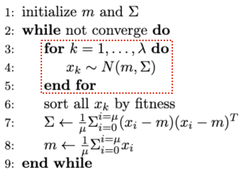
Welcome back! Part 2 & 3 will go over the pseudocode from The CMA Evolution Strategy: A Tutorial page 29. I try to stay on the intuition level and focus on the motivations behind each line. Rest assured! I will not dive too deep into the exact mathematical derivations. Here’s the pseudocode again. I’ll refer to this as the “real CMA-ES” for the rest of this series.

pseudocode from The CMA Evolution Strategy: A Tutorial

If you compare it against our simple ES pseudocode from part 1. The general flows actually have a lot in common. In both pseudocodes, the main loop begins with a section for sampling individuals for the new generation. Let’s see what changes the real CMA-ES makes for the sampling section and why they improve the algorithm.

pseudocode: ES with simple covariance matrix adaptation

What’s new about sampling?

In the real CMA-ES, the sampling is done over three lines. The first line samples from a centered, isotropic normal distribution $N(0, I)$. The second line premultiplies the result with a new term $BD$. The third line scales the premultiplied sample with $\sigma$ and adds back the mean $m$. We see two new terms introduced here: $BD$ and $\sigma$.

Seperating update step size $\sigma$ from update direction $C$

Let’s start with $\sigma$, which is referred to as the overall step size in The CMA Evolution Strategy: A Tutorial p8. It’s important to understand $\sigma$ because it underlies the de-coupling between update step size and update direction in the real CMA-ES. (Please refer to part 1 “An interesting perspective on the role played by covariance matrix” if you are not sure what I mean by update step size and direction) Both update step size and direction used to be controlled by the covariance matrix $\Sigma$ in our simple ES, and thus both were changed alongside one another. However, there are a few reasons against this.

First of all, step size is just a single parameter to be adapted, whereas direction contains multiple parameters; in other words, direction has a larger degree of freedom, and thus is harder to adapt. Intuitively, the adaptation needs to find an exact combination of parameters in order to get a good direction, which is harder than finding just one good value for step size.

Secondly, for a somewhat all-encompassing reason, step size and direction fundamentally leverage different kinds of information for their adaptation. Direction is adapted according to which direction the elites are relative to the current mean, whereas step size is more of a “caution metric” that is adapted according to how successful the past few updates had been (if the past few updates weren’t good, we might be overshooting, so decrease step size). This indicates that we might want different mechanisms for adapting step size and direction.

For a third reason, recall from the end of part 1 that the distribution “size” shrunk too quickly in our simple ES, which used a single $\Sigma$ to control both step size and direction. Actually, we can explain this phenomenon. Consider the variance of the positive half of a univariate normal distribution, i.e. $Var_{new} = Var(max(0, x \sim N(m, Var_{old})))$. Without any calculation, we can already tell $Var_{new} < Var_{old}$, because the range of fluctuation is effectively halved if we only consider the positive half of the distribution. For the same reason, if we estimate the new covariance using only the elites, which tend to cluster on the positive half of the distribution defined by the old covariance, the new covariance will be smaller than the old covariance. What I’m trying to say is, unless if we maintain the scale externally, the covariance matrix tends to “shrink” each time we update it using elites.

I think you should be convinced by now that step size and direction should be adapted seperately. Later in part 3 we will go over pseudocode 43-44 for step size update, and 45-47 for direction update. For now, it suffices to know that in the real CMA-ES, $\Sigma$ is seperated into step size $\sigma$ and direction $C$ such that $\Sigma = \sigma^2 C$.

Think of the new $C$ as a “normalized” covariance matrix that specializes in biasing the samples along a promising direction, and think of the new $\sigma$ as a scaling factor for $C$ that decides how far to explore along that direction.

Eigendecomposition of $C$

The other new term $BD$ originates from the eigendecomposition of $C$, which we just talked about. $B$ is the orthogonal eigenbasis of $C$, and $D^2$ is the corresponding diagonal matrix containing eigenvalues, so we have $C = BD^2B^{-1} = BD^2B^{T}$ ($B^{-1} = B^{T}$ since $B$ is orthogonal). Therefore, $C^{\frac{1}{2}} = BDB^T$.

By premultiplying $z_k \sim N(0, I)$ with $BD$, we get: \(\begin{align*} BDN(0, I) &\sim BDN(0, B^TB) && (B^{T} = B^{-1})\\ &\sim BDB^TN(0, I) && (\text{affine property: } m + AN(0, I) \sim N(m, AA^T))\\ &\sim C^{\frac{1}{2}}N(0, I) \\ &\sim N(0, C) \end{align*}\)

So in short, $BDN(0, I) \sim N(0, C)$. Don’t worry too much about eigendecomposition. To my knowledge, it’s just a faster way to calculate powers of $C$.

Just make sure you understand that the second line of the sampling section, $y_k \sim BDz_k$, combines direction $C$ to the isotropic sampling $z_k \sim N(0, I)$. Then the third line scales $y_k \sim N(0, C)$ with step size $\sigma$, so eventually we get back $\sigma N(0, C) \sim N(0, \sigma^2 C) \sim N(0, \Sigma)$, taking into account both the step size and the direction.

Seperating mean $m$ from sampling

With the de-coupling of $\sigma$ and $C$ explained, we are left with one question about the sampling section: why seperate the mean $m$ from sampling, i.e. why sample $y_k \sim N(0, C)$ and then $x_k \sim m + \sigma y_k$ instead of simply $x_k \sim \sigma N(m, C)$? The reason is that centering the distribution simplifies later calculations. For example, remember that the covariance matrix is calculated with $E[(sample - m)(sample - m)^T]$, but when $m = 0$ as is the case for $y_k \sim N(0, C)$, this simplies to $E[y_k y_k^T]$. So by sampling a centered distribution $y_k \sim N(0, C)$ and then building up to $x_k \sim m + \sigma y_k$, we can use $y_k$ for the covariance matrix calculation, and $x_k$ for the actual individual we feed to the evaluation environment to get back fitness score.

Recombination: updating the mean $m$

The next section of the real CMA-ES updates the mean of the distribution, similar to line 8 from our simple ES. There are just two minor differences.

pseudocode from The CMA Evolution Strategy: A Tutorial

pseudocode: ES with simple covariance matrix adaptation

Firstly, instead of averaging the individuals $x_k \sim \sigma N(m, C) \sim N(m, \Sigma)$ and replacing the old mean with the new, real CMA-ES averages $y_k \sim N(0, C)$, and updates the old mean with the displacement. $c_m$ is the “learning rate” of mean and is a hyperparameter; we can set it to some number within $[0,1]$ to discount the update (if we want to be cautious). I think the mean update from our simple ES would have been just as fine, and the change is purely notational.

Secondly, instead of only considering the elites when averaging, real CMA-ES does a weighted average over all members of the population. Obviously, higher-fitness members are given more weights, so we can use any power-law distribution to get the weights. The real CMA-ES pseudocode uses the function shown below.

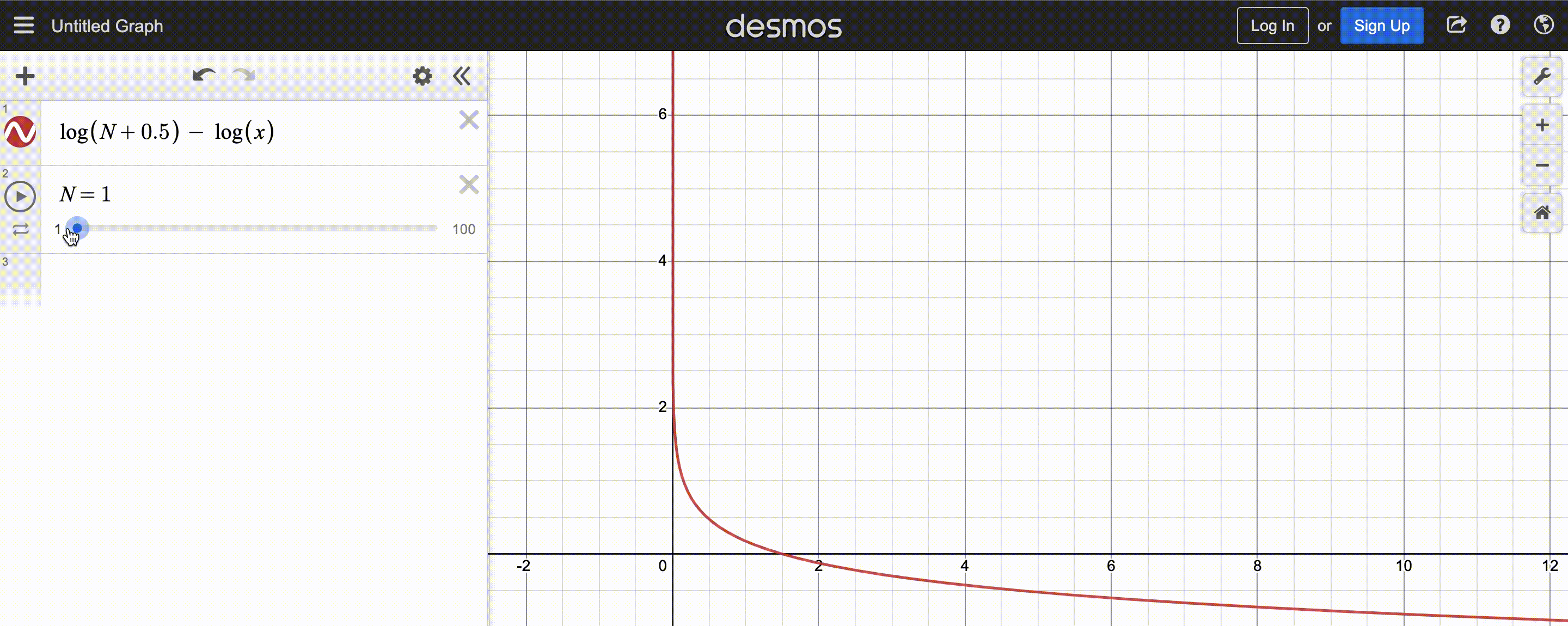power-law function used by CMA-ES; $N$ is population size

After normalizing this function to sum to 1, the y-axis shows the weight and x-axis the fitness rank. You may also observe that the function decays slower for larger population $N$, so there are more positive weights to assign.

Since CMA-ES knows the population size, it can compute the weights at the beginning and store them in a list to be reused each iteration – simply sort the population by fitness, then multiply the first(best) $y_k$ by the first(largest) weight, the second $y_k$ by the second weight, etc.. Optionally, we can even weigh low-fitness $y_k$ by negative weights to discourage reproducing those steps, but the maths get a bit tricky, so I’ll stick to assigning low-fitness $y_k$ very small (but still positive) weights.

That’s it for the recombination section! With the sampling and recombination explained, we only have step size and covariance matrix adaptation sections to cover. Stay tuned for part 3!

Scripts used in this blog can be found at this repo. I also have a (badly recorded) series on Youtube that covers the content in this series.